Leonardo Uieda
Vanderlei C. Oliveira Jr
Valéria C. F. Barbosa


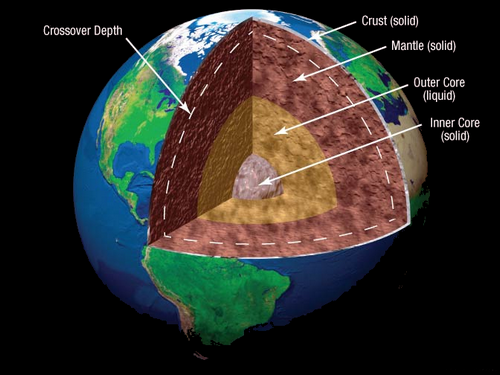
Image credit: http://reinep.wordpress.com
Image credit: http://www.amazon.com/Look-inside-Earth-Poke/dp/0448418908
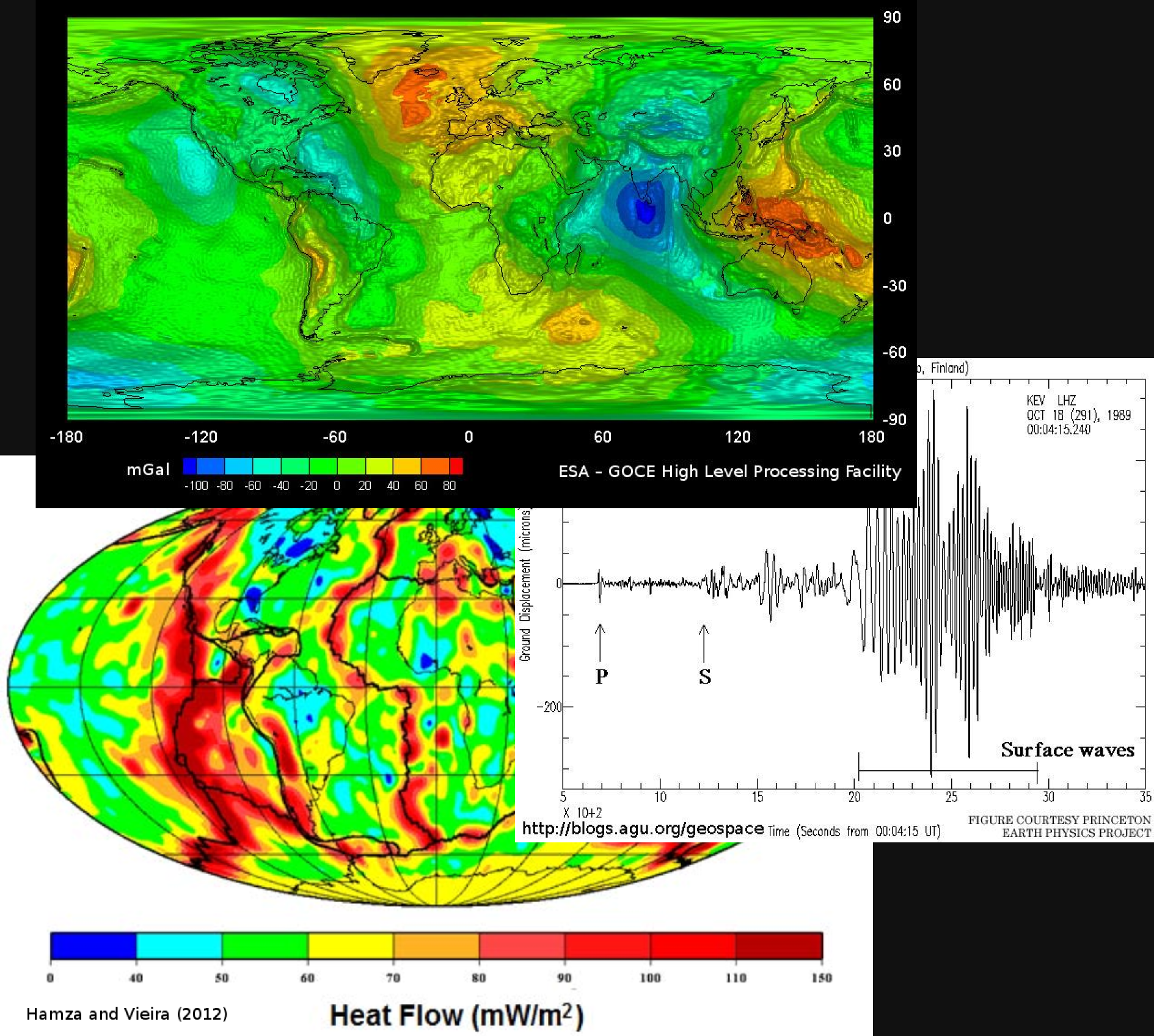
Image credits:
- Gravity field: http://spaceinimages.esa.int/Images/2010/06/GOCE_first_global_gravity_model
- Seismogram: http://blogs.agu.org/geospace/2010/12/17/warning-shaking-rattling-and-rolling-about-to-occur/
- Heat flow: Hamza, V. M., and F. P. Vieira. "Global distribution of the lithosphere-asthenosphere boundary: a new look." Solid Earth 3 (2012): 199-212.
Linear algebra: $\hat{\mathbf{p}} = (\mathbf{G}^T\mathbf{G} + \mu \mathbf{I})^{-1}\mathbf{G}^T\mathbf{d}$
Numerical modeling: differential equations, integration, arrays, etc.
Computation:
for(k = 0; k < glq_lon.order; k++){
    for(j = 0; j < glq_lat.order; j++){
        for(i = 0; i < glq_r.order; i++){
            rc = glq_r.nodes[i];
            sinlatc = sin(d2r*glq_lat.nodes[j]);
            coslatc = cos(d2r*glq_lat.nodes[j]);
            coslon = cos(d2r*(lonp - glq_lon.nodes[k]));
            sinlon = sin(d2r*(glq_lon.nodes[k] - lonp));
            l_sqr = rp*rp + rc*rc - 2*rp*rc*(sinlatp*sinlatc +
                    coslatp*coslatc*coslon);
I/O:
switch(argv[i][1]){
    case 'h':
        if(argv[i][2] != '\0'){
            log_error("invalid argument '%s'", argv[i]);
            bad_args++;
            break;
        }
        print_help();
Custom format (not human readable):
14

16
16
16

0.4 0   0.5

    129.52861   38.6746
    128.88952   25.92015
    130.326     6.44616
    116.52356   -5.8097
    98.09756    -6.64001
- Paraview
- Generic Mapping Tools (GMT)
- Matlab ® (proprietary)
- Surfer ® (proprietary)
Don't get me wrong, these are great software!
"Slicing the Earth"
![]()
Automate
Integrate
API
DRY
Reproduce
def _shapefunc(data, predicted):
    """
    Calculate the total shape of anomaly function between
    the observed and predicted data.
    """
        result = 0.
        for d, p in zip(data, predicted):
            alpha = numpy.sum(d.observed*p)/d.norm**2
            result += numpy.linalg.norm(alpha*d.observed - p)
        return result
Built-in I/O:
- numpy.loadtxt
- pickle
- json
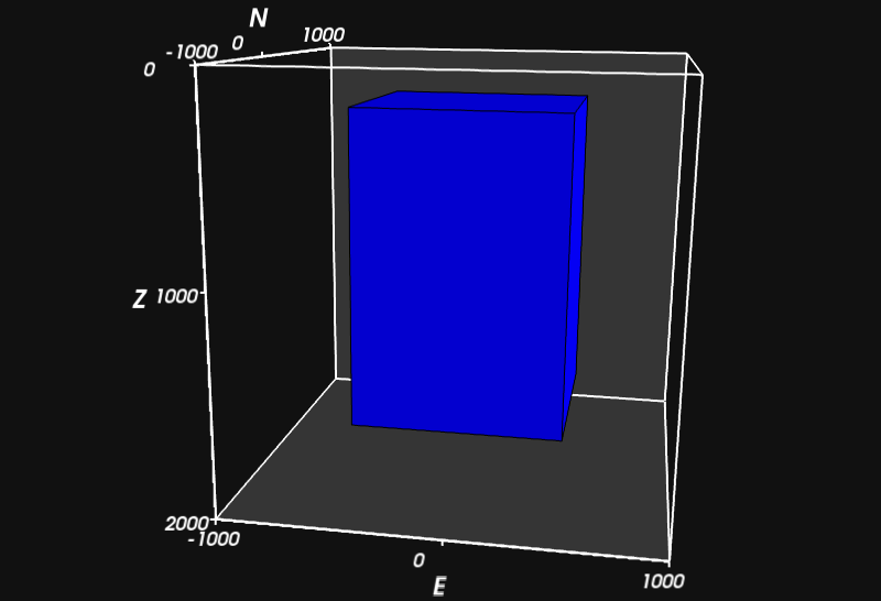
from fatiando import gridder, gravmag
from fatiando.mesher import Prism
model = [Prism(-500,500,-500,500,200,1700,{'density':1000})]
area = [-1000, 1000, -1000, 1000]
bounds = area + [0, 2000]
x, y, z = gridder.scatter(area, 50, z=-1)
g = gravmag.prism.gz(x, y, z, model)
print g.shape, g[:20]
from fatiando.vis import mpl
mpl.figure(figsize=(8, 6))
mpl.axis('scaled')
mpl.contourf(y, x, g, (100, 100), 30, interp=True)
mpl.plot(y, x, '.k')
mpl.colorbar()

from fatiando.vis import myv
f = myv.figure()
gray = (0.066,0.066,0.066); f.scene.background = gray
myv.prisms(model)
wht = (1,1,1)
myv.axes(myv.outline(bounds, color=wht), color=wht)
myv.wall_bottom(bounds, color=wht)
myv.wall_north(bounds, color=wht)
myv.show()
fatiando.gravmag- 3D inversion
- FFT processing
- Modeling
- Equivalent layer
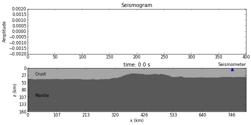
fatiando.seismic- Toy problems
- 2D Finite Differences wave propagation
fatiando.geothermal- Simple temperature log model
fatiando.mesherfatiando.gridderfatiando.utilsfatiando.contantsfatiando.iofatiando.visfatiando.vis.mplfatiando.vis.myv
fatiando.inversion(experimental)
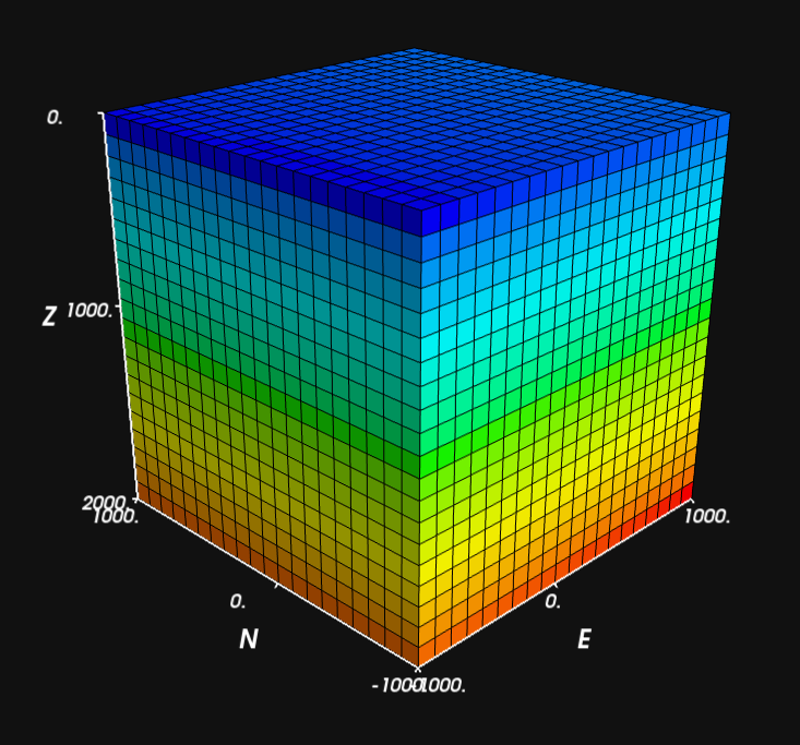
from fatiando.mesher import PrismMesh
mesh = PrismMesh(bounds, (20, 20, 20))
mesh.addprop('density', range(mesh.size))
f = myv.figure(); f.scene.background = gray
p = myv.prisms(mesh, 'density')
myv.axes(p, color=wht); myv.show()
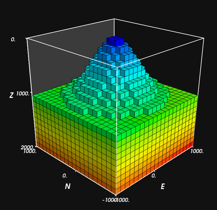
from fatiando import utils
x, y = gridder.regular(bounds[:4], (50, 50))
heights = -1000 + 1000*utils.gaussian2d(x, y, 500, 500)
mesh.carvetopo(x, y, heights)
from fatiando.mesher import Tesseroid
model = [
  Tesseroid(-60,-55,-30,-27,500000,0,{'density':200}),
  Tesseroid(-66,-55,-20,-10,300000,0,{'density':-100})]
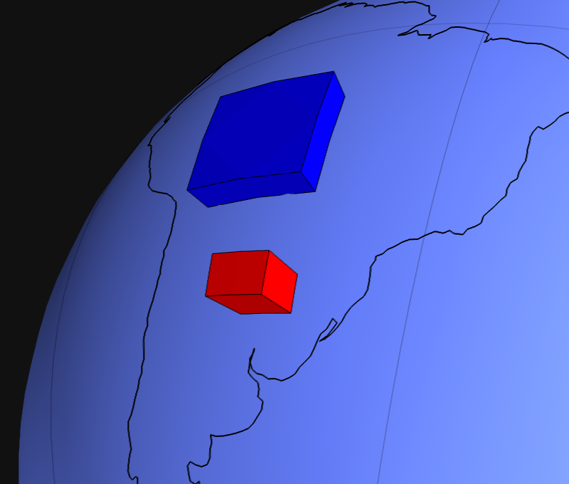
f = myv.figure(zdown=False); f.scene.background = gray
myv.tesseroids(model, 'density')
myv.continents(linewidth=2); myv.earth(opacity=1)
myv.meridians(range(0, 360, 45))
myv.parallels(range(-90, 90, 45))
myv.show()
Calculate gravitational fields (open field of research)
area = [-80, -30, -40, 10]
lons, lats, heights = gridder.scatter(area, 2500, z=2500000)
gz = gravmag.tesseroid.gz(lons, lats, heights, model)
print gz.shape, gz[:30]
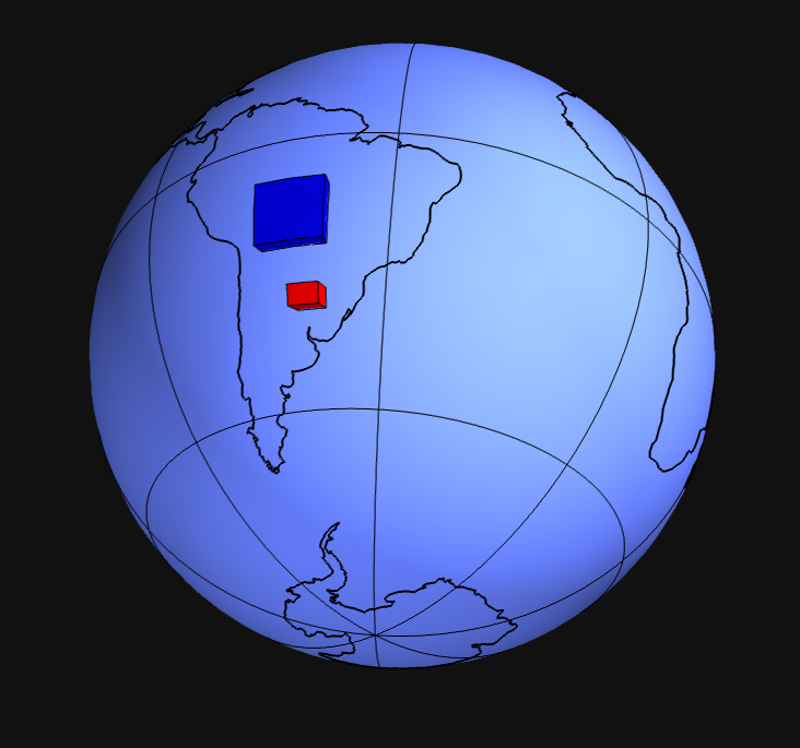
Map projections (with mpl_toolkits.basemap)
mpl.figure(figsize=(8, 6))
bm = mpl.basemap(area, 'ortho')
bm.drawcoastlines(); bm.drawmapboundary()
bm.bluemarble()
mpl.contourf(lons, lats, gz, (50, 50), 30, interp=True, basemap=bm)
mpl.colorbar()


Image credit: http://caitoconnor.blogspot.com/2011/01/ripples.html
from IPython.display import Image
Image(filename="figures/crust.png", width=800)

from fatiando import io
density = io.fromimage('figures/crust.png', ranges=[2700, 3300])
mpl.figure(figsize=(15, 4))
mpl.imshow(density, cmap=mpl.cm.seismic)
cb = mpl.colorbar(shrink=0.6)

- Automate common tasks
- API for modeling
- For teaching and learning
- Use for my own research
- Masters and PhD all included
- Makes my life easier
- Modules available:
- Gravity and magnetic:
fatiando.gravmag - Seismic:
fatiando.seismic - Geothermal:
fatiando.geothermal
- Gravity and magnetic:
- Future:
- More models
- Inverse problem:
fatiando.inversion(experimental) - Improve docs
- Community
- Seismics and Seismology
- Madagascar
- OpendTect
- Obspy
- SAC
- Geodynamics
- Computational Infrastructure for Geodynamics (CIG)
- SEATREE
See Wikipedia for more
Github: github.com/leouieda/fatiando
Slides: github.com/leouieda/scipy2013 (IPython notebook)
Homepage: fatiando.org (blog post coming soon)
from fatiando.mesher import SquareMesh
area = (0, 500000, 0, 500000); shape = (30, 30)
model = SquareMesh(area, shape)
model.img2prop('figures/fatiando-logo.png', 4000, 10000, 'vp')
mpl.figure(figsize=(8, 6)); mpl.axis('scaled')
mpl.squaremesh(model, 'vp', cmap=mpl.cm.seismic)
mpl.colorbar(pad=0.01)
mpl.m2km()

Calculate straight-ray travel times
from fatiando import seismic
quake_locations = utils.random_points(area, 40)
receiver_locations = utils.circular_points(area,
    20, random=True)
quakes, receivers = utils.connect_points(
    quake_locations, receiver_locations)
traveltimes = seismic.ttime2d.straight(model, 'vp',
    quakes, receivers)
noisy = utils.contaminate(traveltimes, 0.1)
print noisy.shape, noisy[:20]
mpl.figure(figsize=(10, 8)); mpl.axis('scaled')
mpl.squaremesh(model, prop='vp', cmap=mpl.cm.seismic)
mpl.paths(quakes, receivers)
mpl.points(quakes, '*y', size=18)
mpl.points(receivers, '^g', size=18)
mpl.m2km()

Run a toy tomography (not for research!)
slowness = seismic.srtomo.run(noisy, quakes, receivers, model, smooth=10**6)[0]
velocity = seismic.srtomo.slowness2vel(slowness)
model.addprop('vp', velocity)
mpl.figure(figsize=(8, 6)); mpl.axis('scaled')
mpl.squaremesh(model, 'vp', cmap=mpl.cm.seismic,
    vmin=4000, vmax=10000)
mpl.colorbar(pad=0.01)
mpl.m2km()
